课程 31 - 图形间的连接关系
在 课程 23 - 思维导图 中,我们仅关注了节点和边的布局算法,并没有深入交互,例如移动节点时绑定的边也要跟着移动。同样在 课程 25 - 绘制箭头 中,直线和箭头的属性中也不包含绑定信息,这节课我们将补全这一点。
数据结构
Excalidraw 中的线性元素
Excalidraw 中,连接线(如箭头)在数据模型中用 ExcalidrawLinearElement 表示,该类型增加了连接相关字段:
export declare type PointBinding = {
    elementId: ExcalidrawBindableElement['id'];
    focus: number;
    gap: number;
};
export declare type ExcalidrawLinearElement = _ExcalidrawElementBase &
    Readonly<{
        type: 'line' | 'arrow';
        points: readonly Point[];
        lastCommittedPoint: Point | null;
        startBinding: PointBinding | null;
        endBinding: PointBinding | null;
        startArrowhead: Arrowhead | null;
        endArrowhead: Arrowhead | null;
    }>;
如上所示,每条箭头具有可选的 startBinding 和 endBinding 字段,它们与 points 处在不同的语义层级,前者为语义约束,而后者 points 为几何表示,当两者同时存在时,points 需要被重新计算。以及起止箭头样式(startArrowhead/endArrowhead)。PointBinding 中的 elementId 指向被连接的图形(可绑定元素,如矩形、椭圆、文本、图片等),focus 和 gap 则用于定位连接点(一个浮点索引和偏移距离)。例如,下面是一个箭头元素在 JSON 中的示例:
{
  "type": "arrow",
  // ... 省略其它属性 ...
  "startBinding": {
    "elementId": "xw25sQBsbd2mecyjTrYHA",
    "focus": -0.0227,
    "gap": 15.6812
  },
  "endBinding": null,
  "points": [[0,0],[0,109]],
  "startArrowhead": null,
  "endArrowhead": null
}
在该例中,箭头的 startBinding 指向 ID 为 "xw25sQBsbd2mecyjTrYHA" 的图形,focus 和 gap 定义了从该图形边界出发的连接位置。
同时,每个被绑定的图形(例如矩形或椭圆)的基本数据结构里有一个 boundElements 列表,用于记录所有连接到它的箭头或文本元素。该字段类型通常为 { id: ExcalidrawLinearElement["id"]; type: "arrow"|"text"; }[] | null。也就是说,箭头与图形之间的连接是双向维护的:箭头记录自己绑定的目标元素 ID,目标元素记录指向它的箭头 ID。
tldraw 中的绑定
在 tldraw 中,“连线”本身也是一种形状(默认是 箭头 形状),其连接关系通过绑定(Binding)对象来表示。每个绑定记录在存储中单独存在,表示两个形状间的关联。对于箭头连接,使用 TLArrowBinding 类型,它是 TLBaseBinding<'arrow',TLArrowBindingProps> 的特化。一个典型的箭头绑定记录示例如下:
{
  id: 'binding:abc123',
  typeName: 'binding',
  type: 'arrow',           // 绑定类型为箭头
  fromId: 'shape:arrow1',  // 箭头形状的ID(箭头形状出发端)
  toId:   'shape:rect1',   // 目标形状的ID(箭头指向的形状)
  props: {
    terminal: 'end',       // 绑定到箭头的哪一端(start 或 end)
    normalizedAnchor: { x: 0.5, y: 0.5 }, // 目标形状上的标准化锚点
    isExact: false,        // 箭头是否进入目标形状内部
    isPrecise: true,       // 是否精确使用锚点,否则使用形状中心
    snap: 'edge',          // 吸附模式(如贴边等)
  },
  meta: {}
}
这里 fromId/toId 字段以形状 ID 的方式关联箭头与目标,props 中存储了连接细节(如锚点、对齐选项等)
antv/g6
连接关系是逻辑的,不是几何的,通过 type 和连线路由算法计算路径:
interface EdgeConfig {
    id?: string;
    source: string; // 源节点 ID
    target: string; // 目标节点 ID

    sourceAnchor?: number; // 源节点锚点索引
    targetAnchor?: number; // 目标节点锚点索引

    type?: string; // line / polyline / cubic / loop ...
    style?: ShapeStyle;
}
在节点上声明锚点,坐标是归一化的:
anchorPoints: [
    [0.5, 0], // top
    [1, 0.5], // right
    [0.5, 1], // bottom
    [0, 0.5], // left
];
在边上使用锚点索引,和 tldraw 的 normalizedAnchor 非常像,但 G6 把锚点定义权放在节点上
{
    source: 'nodeA',
    target: 'nodeB',
    sourceAnchor: 1,
    targetAnchor: 3,
}
mxGraph
mxGraph 有完整的连接约束系统,定义在节点图形上,表示允许连接的点:
class mxConnectionConstraint {
    point: mxPoint | null; // (0.5, 0) = 上中 (1, 0.5) = 右中
    perimeter: boolean; // 表示沿形状边界投射
}
JSON Canvas Spec
Obsidian 开放了 JSON Canvas Spec,结构上和 antv/g6 很类似,在顶层存储了节点和边数组:
{
    "nodes": [],
    "edges": []
}
边的结构如下,不包含几何信息,只有逻辑上的连接关系:
{
    "id": "f67890123456789a",
    "fromNode": "6f0ad84f44ce9c17",
    "toNode": "a1b2c3d4e5f67890"
}
我们的设计
在 Schema 上我们更多参考 mxGraph 的设计。逻辑关系在边上通过 fromId 和 toId 体现,此时就不需要 x1/y1 之类的几何信息。一个连接了 rect-1 和 rect-2 的箭头声明如下:
const edge1 = {
    id: 'line-1',
    type: 'line',
    fromId: 'rect-1',
    toId: 'rect-2',
    stroke: 'black',
    strokeWidth: 10,
    markerEnd: 'line',
};
同时约束关系体现在节点上,类似 mxConnectionConstraint:
interface ConstraintAttributes {
    /**
     * Normalized point, relative to bounding box top-left.
     */
    point: [number, number];
    /**
     * Use perimeter.
     */
    perimeter: boolean;
    name?: string;
    dx?: number;
    dy?: number;
}
类似 课程 18 - 定义父子组件,我们可以实现双向绑定关系:
class Binding {
    @field.ref declare from: Entity;
    @field.ref declare to: Entity;
}

class Binded {
    @field.backrefs(Binding, 'from') declare fromBindings: Entity[];
    @field.backrefs(Binding, 'to') declare toBindings: Entity[];
}
特殊情况
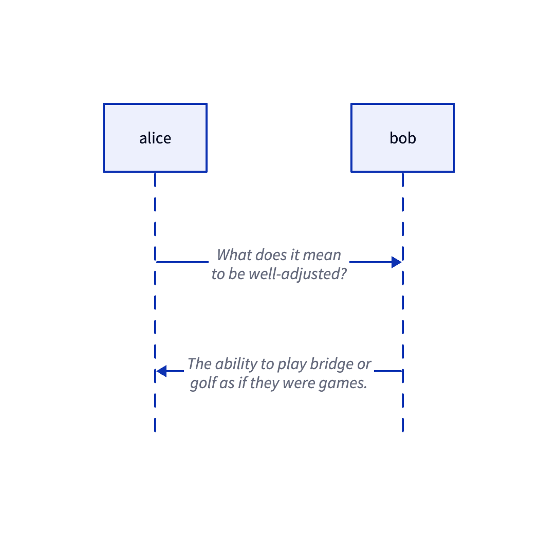
在下一节课中我们会遇到一种特殊情况,即 fromId/toId 可能为空,比如下面顺序图中的虚线,fromId: 'alice', toId: undefined
我们新增一种新的组件,记录仅有一侧关联节点的关系:
/**
 * 仅一端连接图元、另一端由 `sourcePoint` / `targetPoint` 固定的边。
 * `attached` 为已连接侧的实体;`sourceIsAttached === true` 表示连接在 source(`fromId`)侧。
 */
class PartialBinding {
    @field.ref declare attached: Entity;
    /** 1 = source(from)侧连接节点,0 = target(to)侧 */
    @field.int32 declare sourceIsAttached: number;
}
自动更新
当连接的图形位置发生变化时,需要重新计算绑定边的路径。我们可以查询所有持有 Binded 组件的图形,监听它们的包围盒变化,此时更新绑定的边:
class RenderBindings extends System {
    private readonly boundeds = this.query(
        (q) => q.with(Binded).changed.with(ComputedBounds).trackWrites,
    );

    execute() {
        const bindingsToUpdate = new Set<Entity>();
        this.boundeds.changed.forEach((entity) => {
            const { fromBindings, toBindings } = entity.read(Binded);
            [...fromBindings, ...toBindings].forEach((binding) => {
                bindingsToUpdate.add(binding);
            });
        });
        // 重新计算绑定边的路径并渲染
    }
}
在下面的例子中,你可以尝试拖动节点,边会重新计算路径并重绘:
目前边的起点和终点都是被连接图形的包围盒中心,和 tldraw 中 isPrecise 等于 false 时效果一致,表示不精确绑定。 而大多数情况下,我们希望箭头不穿过所连接的图形,而是优雅地停靠在图形边缘。
边界算法
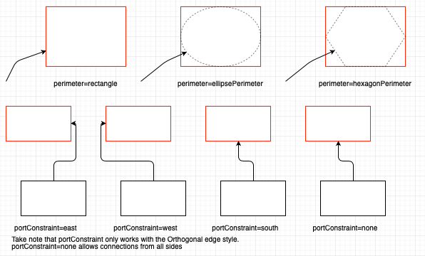
对于图形的边界,drawio 提供了 perimeter 属性,改变它会导致连线,详见:Change the shape perimeter
// 注意一般 next 传入的是“对方中心点”,orthogonal 通常选 false
var pointA = graph.view.getPerimeterPoint(stateA, centerB, false, 0);
var pointB = graph.view.getPerimeterPoint(stateB, centerA, false, 0);
矩形边界算法
矩形的边界算法是最常用的。以下实现中 vertex 为源节点,next 为目标节点的包围盒中心。 首先从源节点和目标节点包围盒的中心做一条连线,然后判断目标点离源节点包围盒的哪条边更近,包围盒的两条对角线将平面划分成了四个区域,左侧边界的范围是 alpha < -pi + t || alpha > pi - t 的判断):
function rectanglePerimeter(
    vertex: SerializedNode,
    next: IPointData,
    orthogonal: boolean,
): IPointData {
    const { x, y, width, height } = vertex;
    const cx = x + width / 2; // 源节点中心
    const cy = y + height / 2;
    const dx = next.x - cx;
    const dy = next.y - cy;
    const alpha = Math.atan2(dy, dx); // 源节点中心到目标节点中心连线的斜率
    const p: IPointData = { x: 0, y: 0 };
    const pi = Math.PI;
    const pi2 = Math.PI / 2;
    const beta = pi2 - alpha;
    const t = Math.atan2(height, width); // 对角线划分了四个区域
    if (alpha < -pi + t || alpha > pi - t) {
        // 与左侧边缘相交
        p.x = x;
        p.y = cy - (width * Math.tan(alpha)) / 2; // 计算交点
    }
    // 省略其他三条边
    return p;
}
最后计算连线与该边的交点作为最终连线的出发点。例如我们确定了连线会经过“左侧边”时:
- 确定
坐标: 既然是左边缘,交点的 坐标必然等于矩形的左边界值 vertex.x。 - 计算
偏移量: - 从中心到左边缘的水平距离是 width / 2。
- 利用正切公式:
。 - 在左侧,
。 - 所以垂直偏移量
。
- 最终坐标:
p.y = cy + Δy,即代码中的cy - (width * Math.tan(alpha)) / 2。
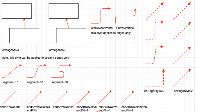
draw.io 还提供了另一个选项 orthogonal,表示计算的线需要正交对齐(即与 x 或 y 轴对齐),线只考虑水平或垂直延伸。此时就不能使用对方的中心点作为参考了:
if (orthogonal) {
    if (next.x >= x && next.x <= x + width) {
        p.x = next.x;
    } else if (next.y >= y && next.y <= y + height) {
        p.y = next.y;
    }
    if (next.x < x) {
        p.x = x;
    } else if (next.x > x + width) {
        p.x = x + width;
    }
    if (next.y < y) {
        p.y = y;
    } else if (next.y > y + height) {
        p.y = y + height;
    }
}
椭圆边界算法
对于椭圆节点,需要计算直线和它的交点:
const d = dy / dx;
const h = cy - d * cx;
const e = a * a * d * d + b * b;
const f = -2 * cx * e;
const g = a * a * d * d * cx * cx + b * b * cx * cx - a * a * b * b;
const det = Math.sqrt(f * f - 4 * e * g);

const xout1 = (-f + det) / (2 * e);
const xout2 = (-f - det) / (2 * e);
const yout1 = d * xout1 + h;
const yout2 = d * xout2 + h;
const dist1 = Math.sqrt(Math.pow(xout1 - px, 2) + Math.pow(yout1 - py, 2));
const dist2 = Math.sqrt(Math.pow(xout2 - px, 2) + Math.pow(yout2 - py, 2));

let xout = 0;
let yout = 0;
if (dist1 < dist2) {
    xout = xout1;
    yout = yout1;
} else {
    xout = xout2;
    yout = yout2;
}
return { x: xout, y: yout };
连线经过中心
- 斜率
- 截距
将直线方程代入椭圆标准方程:
展开并整理成关于
: 二次项系数 : 一次项系数 : 常数项
求根公式: 使用判别式
定义约束
至此,我们实现了在边上仅通过 fromId 和 toId 表达逻辑连接关系的实现。边和节点的连接点是浮动的,在 mxGraph 中称作 FloatingTerminalPoint。但有时我们希望边从节点的固定位置离开、从被连接图形的固定位置进入,在 mxGraph 称作 FixedTerminalPoint,此时就需要通过约束定义,分成节点和边两部分。
节点约束
节点约束表示允许你从哪些位置、以什么规则连线,它不是一个“点”,而是一个规则对象,在 mxGraph 中定义如下:
class mxConnectionConstraint {
    point: mxPoint | null; // 归一化坐标 (0~1)
    perimeter: boolean; // 是否投射到边界
    name?: string; // 可选,端口名
}
在配套的 draw.io 的编辑器中我们能看到图形上许多“蓝色连接点”,它们就是通过重载图形上的约束定义的:
mxRectangleShape.prototype.getConstraints = function (style) {
    return [
        new mxConnectionConstraint(new mxPoint(0.5, 0), true), // top
        new mxConnectionConstraint(new mxPoint(1, 0.5), true), // right
        new mxConnectionConstraint(new mxPoint(0.5, 1), true), // bottom
        new mxConnectionConstraint(new mxPoint(0, 0.5), true), // left
    ];
};
我们的约束定义如下,在节点上可以声明一组约束:
export interface ConstraintAttributes {
    x?: number;
    y?: number;
    perimeter?: boolean;
    dx?: number;
    dy?: number;
}

export interface BindedAttributes {
    constraints: ConstraintAttributes[];
}
获取候选约束,选择最近的约束,将约束转为几何点。如果需要投射到边界,就进入上一节介绍过的边界算法计算逻辑。
边约束
在边上也需要定义从节点的哪个锚点上离开或进入,在交互操作上对应将边的端点拖拽到节点的锚点上,此时 entryX/entryY 就需要拷贝锚点约束的 x/y 字段:
interface BindingAttributes {
    fromId: string;
    toId: string;
    orthogonal: boolean;
    exitX: number;
    exitY: number;
    exitPerimeter: boolean;
    exitDx: number;
    exitDy: number;
    entryX: number;
    entryY: number;
    entryPerimeter: boolean;
    entryDx: number;
    entryDy: number;
}
在下面的例子中,我们分别在灰色和绿色矩形上各定义了一个锚点 [1, 0] 和 [0, 1]
路由规则
mxGraph 使用 EdgeStyle 函数来实现路由规则,这些函数负责:
- 自动选择出口方向
- 插入拐点(Waypoints)
- 避开节点包围盒
- 计算正交/直角路径
| 连接器 | 特点 | 适用场景 |
|---|---|---|
| OrthConnector | 自动生成正交边,支持复杂约束 | 流程图、组织结构图等自动生成布局 |
| SegmentConnector | 支持用户自定义控制点,灵活可交互 | 用户需要手动调整正交边的路径 |
| ElbowConnector | 单个 L 形转折点 | 简单的 2 段路径(例如面包屑导航) |
| SideToSide | 水平方向优先的连接 | 源和目标节点水平分布 |
| TopToBottom | 垂直方向优先的连接 | 源和目标节点垂直分布 |
| EntityRelation | 数据库关系图专用,生成灵活的路径 | 数据库 ER 图,双向关系 |
| Loop | 实现自环连接 | 状态图或自动机图表的自循环关系 |
OrthConnector
OrthConnector 是最常见的路由算法,核心目标是在源节点和目标节点之间创建一条只包含水平和垂直线段的路径,避免斜线。具体步骤如下:
- 确定源和目标的出口/入口方向
- 根据方向组合查找预定义路由模式
- 应用路由模式生成拐点序列
- 处理避障和优化
┌──────┐        ┌──────┐
│ Node │ ─┐     │ Node │
└──────┘  └────▶└──────┘
确定出入口方向
先来看无任何端口约束的情况。首先需要确定目标相对于源的象限位置,通过比较两者的几何中心点可得:
// 0 | 1
// -----
// 3 | 2

let dx = sourceCenX - targetCenX;
let dy = sourceCenY - targetCenY;
let quad = 0;
if (dx < 0) {
    if (dy < 0) {
        quad = 2;
    } else {
        quad = 1;
    }
}
// 省略其他情况
接下来是最复杂的部分,确定边应该从哪个方向离开源节点和进入目标节点。
首先计算节点间的距离:
        sourceTopDist
             ↑
    [Source] |
             ↓
        sourceBottomDist
             ↑
             | [Target]

sourceLeftDist ← [Source] → sourceRightDist → [Target]
然后确定首选方向,采用选择空间更大的方向的策略:
- 如果左侧距离 ≥ 右侧距离,源节点首选向西(左)
- 如果顶部距离 ≥ 底部距离,源节点首选向北(上)
- 目标节点的首选方向是源节点的相反方向
var dirPref = [];
var horPref = [];
var vertPref = [];

horPref[0] =
    sourceLeftDist >= sourceRightDist
        ? mxConstants.DIRECTION_MASK_WEST
        : mxConstants.DIRECTION_MASK_EAST;
vertPref[0] =
    sourceTopDist >= sourceBottomDist
        ? mxConstants.DIRECTION_MASK_NORTH
        : mxConstants.DIRECTION_MASK_SOUTH;

horPref[1] = mxUtils.reversePortConstraints(horPref[0]);
vertPref[1] = mxUtils.reversePortConstraints(vertPref[0]);

var preferredHorizDist =
    sourceLeftDist >= sourceRightDist ? sourceLeftDist : sourceRightDist;
var preferredVertDist =
    sourceTopDist >= sourceBottomDist ? sourceTopDist : sourceBottomDist;
路由模式选择
根据源和目标的方向索引,从预定义的 routePatterns 中选择路由模式来保证质量,使用位掩码编码:
- 低 4 位:方向(1=西, 2=北, 4=东, 8=南)
- 第 5-8 位:边的哪一侧
- 第 9 位:是否使用中心点
- 第 10 位:是否关联源节点
- 第 11 位:是否关联目标节点
routePatterns: [
    [ [ 513, 2308, 2081, 2562 ], [ 513, 1090, 514, 2184, 2114, 2561 ],
        [ 513, 1090, 514, 2564, 2184, 2562 ],
        [ 513, 2308, 2561, 1090, 514, 2568, 2308 ] ],
    // ... 更多模式
],
生成实际路径点
遍历路由模式,根据方向生成实际的路径点。
for (var i = 0; i < routePattern.length; i++)
{
    var nextDirection = routePattern[i] & 0xF;

    // Rotate the index of this direction by the quad
    var directionIndex = nextDirection == mxConstants.DIRECTION_MASK_EAST ? 3
            : nextDirection;

    directionIndex += quad;

    if (directionIndex > 4)
    {
        directionIndex -= 4;
    }
最后优化路径中距离很近的相邻点,这部分我们继续使用 simplify-js,在 课程 12 - 简化折线的顶点 中已经介绍过了。
SegmentConnector
OrthConnector 更偏自动路由,当用户显式指定了控制点 controlHints 时,SegmentConnector 会把 hints 变成“必须经过/对齐”的拐点,最终折线基本围绕这些 hints 构造,因此它更可预测、交互编辑体验更一致。
LoopConnector
当起点和终点重合时,就需要创建自环了。
连接线样式
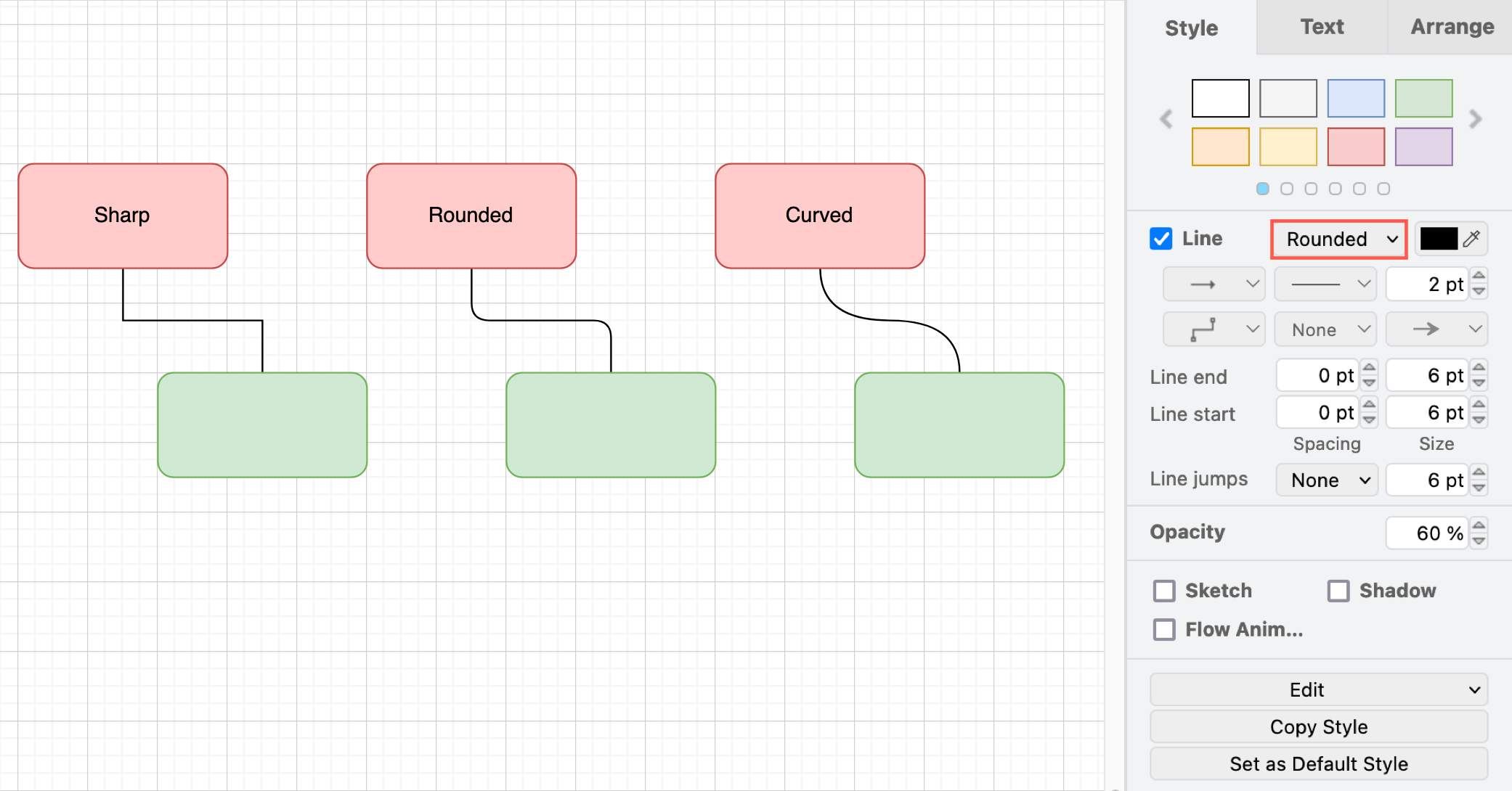
圆角
圆角效果的本质是:仍然是使用之前计算的折线实际路径点,但在连接处用圆角过渡替换尖角。具体步骤如下:
- 遍历每个折线拐点
- 在拐点两侧各“退开”一段距离(不超过线段一半)
- 用 quadTo(或等价曲线指令)在拐角处画一段圆滑过渡。
二次贝塞尔曲线
使用二次贝塞尔曲线连接相邻的控制点:
const p0 = pts[n - 2];
const p1 = pts[n - 1];
parts.push(
    `Q ${formatNumber(p0.x)} ${formatNumber(p0.y)} ${formatNumber(
        p1.x,
    )} ${formatNumber(p1.y)}`,
);
三次贝塞尔曲线
满足 3n+1 的情况下,则按 [anchor, cp1, cp2, anchor, ...] 直接把连接点点解释为三次贝塞尔控制点,否则退化成二次贝塞尔曲线。
if ((n - 1) % 3 === 0) {
    for (let i = 1; i + 2 < n; i += 3) {
        const cp1 = pts[i];
        const cp2 = pts[i + 1];
        const end = pts[i + 2];
        parts.push(
            `C ${formatNumber(cp1.x)} ${formatNumber(cp1.y)} ` +
                `${formatNumber(cp2.x)} ${formatNumber(cp2.y)} ` +
                `${formatNumber(end.x)} ${formatNumber(end.y)}`,
        );
    }
    return parts.join(' ');
}
[WIP] 导出 SVG
在导出时,就不能只保存几何信息了,还需要将逻辑关系也一并持久化。例如 drawio 在导出时会将原始 mxfile 内容也保存到 <svg> 的 content 属性(这并不是规范的一部分)中:
<svg content='<mxfile host="app.diagrams.net" diagram name="Page-1"'></svg>我们也可以将
<line x1="0" y1="0" data-binding="" />编辑器
高亮锚点
- 选中节点时,展示可用的锚点,从锚点可以发起连线。
- 选中边时,拖拽时高亮可停靠的锚点。